The average of a set of data is typically defined as the sum of the values divided by the number of data points. But what if you have infinitely many data points? What is the average value of a function? Read on to find out!
Average Value of Functions
Suppose f is a continuous function defined over an interval [a, b]. In particular f(x) exists at every one of the infinitely-many points x between and including a and b. So, if you’re looking for the average value of f on that interval, it won’t do any good to try adding up those infinitely-many data points.
Instead, the way to tame the infinity is to use calculus. Specifically, we define the average value of a function f as the following definite integral.
![]()
The Theory Behind the Formula
But where does the integral formula for average come from?
The key is sampling. If you included enough of the function values, say a thousand, a million, or even more, then that should approximate the average of all infinitely-many points!
Let’s illustrate with the following example.
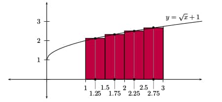
Estimate the average value of the function f(x) = √(x) + 1 over the interval [1, 3].
Since we’re just estimating, let’s pick four sample points. (The more sample points you pick, the better your estimated average will be.)
Divide the interval [1, 3] into four equal subintervals, and let’s agree to choose the midpoint of each subinterval. Then plug those midpoints into f to find the sample values.
| Midpoints | Height: f(x) = √(x) + 1 |
|---|---|
| 1.25 | √(1.25) + 1 = 2.12 |
| 1.75 | √(1.75) + 1 = 2.32 |
| 2.25 | √(2.25) + 1 = 2.50 |
| 2.75 | √(2.75) + 1 = 2.66 |
Finally, use the familiar old averaging formula. Add up the data and divide by the number of data points:
(2.12 + 2.32 + 2.50 + 2.66)/4 = 2.4
So the (approximate) average of the function is 2.4.
Taking it to the Limit
However, what we’ve just done will not give us an exact answer because we’ve essentially ignored most of the function! What about f(1.3) or f(2.95234)? No matter how many sample points we include, there will always be some missing… Unless we can use the magic of calculus to catch them all.
The sampling process should remind you of a Riemann Sum. For a quick reminder, feel free to check out AP Calculus Review: Riemann Sums.
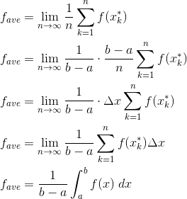
Let n be any whole number and xk* stand for the various sample x-values. Then the estimated average is the sum:

Next, allow n → ∞ using a limit. We also need to get Δx into the act somehow. The trick is to multiply and divide by (b – a). Remember, Δx = (b – a)/n.
Examples
Ok, now that you’ve seen the theory, let’s use the formula in practice!
Problem 1
Find the exact average value of f(x) = √(x) + 1 over the interval [1, 3].
Solution
Above, we only estimated the average to be 2.4. Now we’ll use the integral formula to determine the average value precisely.
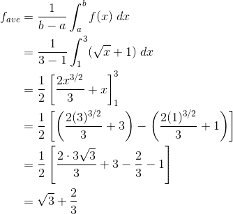
(It’s interesting to compare our estimate with the exact value above. √(3) + 2/3 ≈ 2.39871747, which means that our estimate of 2.4 was actually pretty good!)
Problem 2
The amount of energy associated with a certain chemical reaction is given by E = x ln x, where 1 ≤ x ≤ e, and x represents the amount of one of the reactants. Find the average energy of the reaction over the range of possible levels of reactant.
Solution
This problem seems more like chemistry than math!

However, the keyword average tells us that mathematics plays a major role in this problem. In fact, they are simply asking for the average value of f(x) = x ln x, over the interval [1, e].
First set up the integral formula with a = 1 and b = e. Then work out the integration, which involves Integration By Parts in this case.
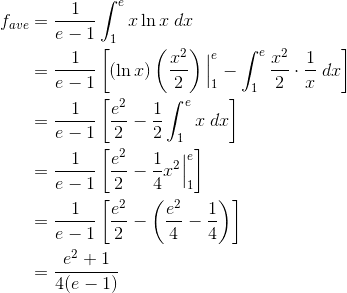
Thus the average energy of the reaction is (e2 + 1)/[ 4(e – 1) ], or roughly 1.22.
Mean Value Theorem for Integrals
Averages are also called means. So you may use the same formula to find the mean value of a function.
There is also an important result in calculus that relates the mean value to a particular function value on the given interval.
The Mean Value Theorem for Integrals (MVTI). If f is continuous on a closed interval [a, b], then there is at least one point x = c in that interval such that the mean value of the function is equal to f(c). That is,
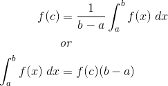
(Caution: There is also a Mean Value Theorem for Derivatives. It’s important not to confuse the two.)
Problem 3
Let f(x) = 6x2 – 8x + 1. Determine the value of c at which the mean value of f on [-1, 1] is the same as f(c).
Solution
According to the Mean Value Theorem for Integrals, there must be at least one such value c. Let’s set up the formula and find it!
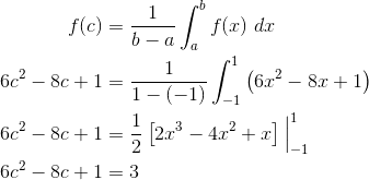
At this point, we will need to solve a quadratic equation. Don’t forget your Quadratic Formula!
6c2 – 8c – 2 = 0
c = (2 ± √(7))/3
It seems as though there may be two answers. However, only one lies within the given interval [-1, 1].
c = (2 + √(7))/3 ≈ 1.549, not in the interval.
c = (2 – √(7))/3 ≈ -0.215, in the interval.
Therefore, the only value that satisfies the MVTI is c = (2 – √(7))/3.
Summary
Although average value and the Mean Value Theorem for Integrals are specialized topics and only show up in a few problems on any given AP Calculus test, they are important concepts to master. For one thing, they illustrate how integral calculus can be used in applications.
Moreover, working out the average value of a function is no more difficult than computing a definite integral. So now when you see these kinds of problems on the AP Calculus Exam, you can rise to the challenge!


Leave a Reply