What is linear approximation? Basically, it’s a method from calculus used to “straighten out” the graph of a function near a particular point. Scientists often use linear approximation to understand complicated relationships among variables.
In this review article, we’ll explore the methods and applications of linear approximation. We’ll also take a look at plenty of examples along the way to better prepare you for the AP Calculus exams.
Linear Approximation and Tangent Lines
By definition the linear approximation for a function f(x) at a point x = a is simply the equation of the tangent line to the curve at that point. And that means that derivatives are key! (Check out How to Find the Slope of a Line Tangent to a Curve or Is the Derivative of a Function the Tangent Line? for some background material.)
Formula for the Linear Approximation
Given a point x = a and a function f that is differentiable at a, the linear approximation L(x) for f at x = a is:
L(x) = f(a) + f '(a)(x – a)
The main idea behind linearization is that the function L(x) does a pretty good job approximating values of f(x), at least when x is near a.
In other words, L(x) ≈ f(x) whenever x ≈ a.
Example 1 — Linearizing a Parabola
Find the linear approximation of the parabola f(x) = x2 at the point x = 1.
A. x2 + 1
B. 2x + 1
C. 2x – 1
D. 2x – 2
Solution
C.
Note that f '(x) = 2x in this case. Using the formula above with a = 1, we have:
L(x) = f(1) + f '(1)(x – 1)
L(x) = 12 + 2(1)(x – 1) = 2x – 1
Follow-Up: Interpreting the Results
Clearly, the graph of the parabola f(x) = x2 is not a straight line. However, near any particular point, say x = 1, the tangent line does a pretty good job following the direction of the curve.
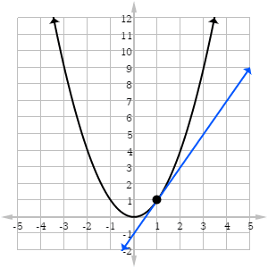
How good is this approximation? Well, at x = 1, it’s exact! L(1) = 2(1) – 1 = 1, which is the same as f(1) = 12 = 1.
But the further away you get from 1, the worse the approximation becomes.
| x | f(x) = x2 | L(x) = 2x – 1 |
|---|---|---|
| 1.1 | 1.21 | 1.2 |
| 1.2 | 1.44 | 1.4 |
| 1.5 | 2.25 | 2 |
| 2 | 4 | 3 |
Approximating Using Differentials
The formula for linear approximation can also be expressed in terms of differentials. Basically, a differential is a quantity that approximates a (small) change in one variable due to a (small) change in another. The differential of x is dx, and the differential of y is dy.
Based upon the formula dy/dx = f '(x), we may identify:
dy = f '(x) dx
The related formula allows one to approximate near a particular fixed point:
f(x + dx) ≈ y + dy
Example 2 — Using Differentials With Limited Information
Suppose g(5) = 30 and g '(5) = -3. Estimate the value of g(7).
A. 24
B. 27
C. 28
D. 33
Solution
A.
In this example, we do not know the expression for the function g. Fortunately, we don’t need to know!
First, observe that the change in x is dx = 7 – 5 = 2.
Next, estimate the change in y using the differential formula.
dy = g '(x) dx = g '(5) · 2 = (-3)(2) = -6.
Finally, put it all together:
g(5 + 2) ≈ y + dy = g(5) + (-6) = 30 + (-6) = 24
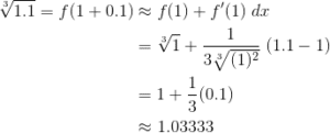
Example 3 — Using Differentials to Approximate a Value
Approximate ![]() using differentials. Express your answer as a decimal rounded to the nearest hundred-thousandth.
using differentials. Express your answer as a decimal rounded to the nearest hundred-thousandth.
Solution
1.03333.
Here, we should realize that even though the cube root of 1.1 is not easy to compute without a calculator, the cube root of 1 is trivial. So let’s use a = 1 as our basis for estimation.
Consider the function ![]() . Find its derivative (we’ll need it for the approximation formula).
. Find its derivative (we’ll need it for the approximation formula).
![]()
Then, using the differential, ![]() , we can estimate the required quantity.
, we can estimate the required quantity.
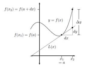
Exact Change Versus Approximate Change
Sometimes we are interested in the exact change of a function’s values over some interval. Suppose x changes from x1 to x2. Then the exact change in f(x) on that interval is:
Δy = f(x2) – f(x1)
We also use the “Delta” notation for change in x. In fact, Δx and dx typically mean the same thing:
Δx = dx = x2 – x1
However, while Δy measures the exact change in the function’s value, dy only estimates the change based on a derivative value.
Example 4 — Comparing Exact and Approximate Values
Let f(x) = cos(3x), and let L(x) be the linear approximation to f at x = π/6. Which expression represents the absolute error in using L to approximate f at x = π/12?
A. π/6 – √2/2
B. π/4 – √2/2
C. √2/2 – π/6
D. √2/2 – π/4
Solution
B.
Absolute error is the absolute difference between the approximate and exact values, that is, E = | f(a) – L(a) |.
Equivalently, E = | Δy – dy |.
Let’s compute dy ( = f '(x) dx ). Here, the change in x is negative. dx = π/12 – π/6 = -π/12. Note that by the Chain Rule, we obtain: f '(x) = -3 sin(3x). Putting it all together,
dy = -3 sin(3 π/6 ) (-π/12) = -3 sin(π/2) (-π/12) = 3π/12 = π/4
Ok, next we compute the exact change.
Δy = f(π/12) – f(π/6) = cos(π/4) – cos(π/2) = √2/2
Lastly, we take the absolute difference to compute the error,
E = | √2/2 – π/4 | = π/4 – √2/2.
Application — Finding Zeros
Linear approximations also serve to find zeros of functions. In fact Newton’s Method (see AP Calculus Review: Newton’s Method for details) is nothing more than repeated linear approximations to target on to the nearest root of the function.
The method is simple. Given a function f, suppose that a zero for f is located near x = a. Just linearize f at x = a, producing a linear function L(x). Then the solution to L(x) = 0 should be fairly close to the true zero of the original function f.
Example 5 — Estimating Zeros
Estimate the zero of the function ![]() using a tangent line approximation at x = -1.
using a tangent line approximation at x = -1.
A. -1.48
B. -1.53
C. -1.62
D. -1.71
Solution
D.
Remember, The purpose of this question is to estimate the zero. First of all, the tangent line approximation is nothing more than a linearization. We’ll need to know the derivative:
![]()
Then find the expression for L(x). Note that g(-1) ≈ 2.13 and g '(-1) = 3.
L(x) = 2.13 + 3(x – (-1)) = 5.13 + 3x.
Finally to find the zero, set L(x) = 0 and solve for x
0 = 5.13 + 3x → x = -5.13/3 = -1.71