
The Mean Value Theorem may seem at first like an esoteric result with no practical application. However in this article I hope to show you that it’s not as abstract as it sounds.
The Mean Value Theorem
First, let’s see what the precise statement of the theorem is.
- The Mean Value Theorem (MVT). Suppose f is a function that is continuous on [a, b] and differentiable on (a, b). Then there is at least one value x = c such that a < c < b and

Note, this is the MVT for Derivatives (MVTD). There is also a Mean Value Theorem for Integrals (MVTI), which we do not cover in this article.
The final equation can be interpreted as follows:
There is at least one point c in the interval at which the instantaneous rate of change f ‘(c) is the same as the average rate of change [f(b) – f(a)]/[b – a].
Let’s try to understand this result by way of a more familiar example.
Average vs. Instantaneous Velocity
Suppose you take a road trip from Amarillo (Texas) to Albuquerque (New Mexico). According to the map, the shortest route is about 286 miles. Now suppose you arrive in Albuquerque exactly 4 hours after leaving Amarillo. What was your average speed?

Of course you know that speed (or velocity) is a measure of distance per time. So you can compute your average speed to be about 286/4 = 71.5 miles per hour.
Does this mean that your car was always traveling at 71.5 mph? Probably not. But we can be sure that the speedometer did hit 71.5 at least once during the trip.
Here’s how we know. The car could not have been going less than 71.5 the entire trip; otherwise the average speed would be lower than 71.5. Conversely, the car could not have always had a speed above 71.5.
So the car sometimes would go less than 71.5 mph, and sometimes greater than 71.5. If at some point in time the car was going, say 70 mph, and at a later time going maybe 75, then it had to have hit 71.5 for at least an instant as the speedometer crept upwards from 70 to 75, right?
This is really the essence of the MVT. There must have been at least one point in time during the trip when the instantaneous velocity matched the average velocity.
Secants and Tangents
Another way to interpret the Mean Value Theorem is to think in terms of slope.
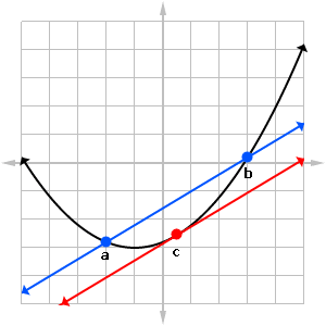
The right hand side of the MVT equation is nothing more than a slope calculation. Imagine a line drawn through the two points (a, f(a)) and (b, f(b)) on the graph of f. This is called a secant line. In fact the term secant line refers to any line drawn between two given points on a graph.
What is the slope of this secant line? Using the slope formula with x1 = a, y1 = f(a), x2 = b, and y2 = f(b), we get:
![]()
On the other side of the coin, the left hand side of the MVT equation is simply the derivative evaluated at some unspecified point c. And we know that the derivative measures the slope of the tangent line through any given point.
What the MVT is saying is that as long as f is continuous on [a, b] and differentiable on (a, b), then there must be a tangent line at some point c which is parallel to the secant line connecting (a, f(a)) and (b, f(b)) on the graph.
Sample Problem 1
Find all values c that satisfy the Mean Value Theorem for f(x) = x3 + 3x2 – 2x + 1 on [-5, 3].
Solution
First check whether this function satisfies the hypotheses of the MVT on the given interval. Because f is a polynomial, it’s continuous everywhere, so in particular f is continuous on [-5, 3].
Furthermore, since f ‘(x) = 3x2 + 6x – 2 is also polynomial, the derivative exists everywhere. In particular, f is differentiable on (-5, 3).
Therefore, by the MVT, there must be at least one value x = c with -5 < c < 3 such that
![]()
Now let’s plug in a = -5 and b = 3 and work out the unknown value of c.
Note, f(-5) = -39 and f(3) = 49 can be found by evaluating the original function at the given endpoints.
Use the quadratic equation to solve for the unknown values of c.
![]()
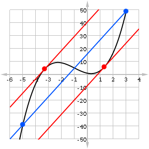
Here we find two values, c ≈ -3.3094 and 1.3094, both of which are in the interval.
It’s interesting to take a look at the graph and note that there are indeed two points where the tangent line must be parallel to the secant line.
Rolle’s Theorem
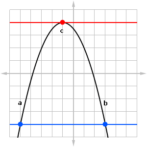
There is a special case of the Mean Value Theorem called Rolle’s Theorem. Basically, Rolle’s Theorem is the MVT when slope is zero.
- Rolle’s Theorem. Suppose f is a function that is continuous on [a, b] and differentiable on (a, b). If f(a) = f(b), then there is at least one value x = c such that a < c < b and f ‘(c) = 0.
Graphically, Rolle’s Theorem states that if two function values are the same, then somewhere in between them there must exist a horizontal tangent.
Sample Problem 2
Prove that the function f(x) = sin 3x cos 5x has at least one critical number in the interval (0, π/10).
Solution
Finding the critical number(s) directly would be extremely difficult. Fortunately, the question does not ask for the exact values of the critical numbers. Instead we will use Rolle’s Theorem to prove that at least one must exist.
First, since f is a product of a sine and cosine function, it is continuous and differentiable everywhere.
Next, check the value of f at the endpoints.
f(0) = sin(0) cos(0) = 0.
f(π/10) = sin(3π/10) cos(π/2) = sin(3π/10) × 0 = 0.
Since f(0) = f(π/10), Rolle’s Theorem implies that there is at least one point x = c between 0 and π/10 such that f ‘(c) = 0. In other words, there is at least one critical number on the interval (0, π/10).
Final Thoughts
Both the MVT and Rolle’s Theorem are existence theorems. They tell us under what conditions a certain thing is guaranteed to exist, but they do not tell us exactly how to find it. For this reason, the theorems can be tricky to interpret and to apply in problems.
However, as long as you know the hypotheses and conclusion of the two theorems, you should have no trouble when asked about them on the AP Calculus AB and BC exams!


Leave a Reply