
Taylor polynomials are certain polynomials that can approximate functions. The more terms in the Taylor polynomial, the greater the accuracy of the approximation.

In this article we will define Taylor polynomials and work out a number of examples similar to those you might see on the AP Calculus BC exam.
Taylor Polynomials
Before we define the Taylor polynomial, let’s remember what a normal, everyday kind of polynomial is.
Polynomials
A polynomial is any expression of the following form.
![]()
Here, n is a whole number. Each coefficient a0, a1, a2, …, an, must be constant. Furthermore, we always insist that an is nonzero. (Otherwise, we really wouldn’t have an nth term at all, right?) Then we say that the degree of the polynomial is n.
Often, you’ll see the terms written in the opposite order, from high degree down to low, which is called standard form. But a Taylor polynomial is usually written starting from low degree and then progressing to higher degrees with each term. However you slice it, a polynomial is simply the sum of a terms, each of which involving a whole number power of the variable.
Here are a few example polynomials:
![]()
![]()
![]()
Here, f has degree 6, g has degree 8, and h has degree 11.
Polynomials and Derivatives
The nice thing about a polynomial is that it’s very easy to take its derivative. All you need are three simple rules.
- The Sum/Difference Rule

- the Constant Multiple Rule

- and the Power Rule

Now, even if you replace x by (x – c) in a polynomial, you still get a polynomial. Let’s explore the derivatives of such a function.
As you keep taking higher-order derivatives, notice how the degree of the polynomial steps down.
Another curiousity is how the constant terms behave. By plugging x = c into the function and each successive derivative, you can recover each constant term. Take a look at the pattern that emerges.
- Original function: f(c) = a0
- First derivative: f '(c) = a1
- Second derivative: f ''(c) = 2a2
- Third derivative: f '''(c) = 6a3
By the time you get all the way to the nth derivative, there’s nothing left but the last term. Each derivative step tacks on another factor, until you end up with all of the counting numbers starting from n down to 1 multiplied to the final coefficient:
![]()
You might recognize that “excited” notation, n!, as the factorial of n.
Taylor Coefficients
Now I bet you’re wondering what all of this have to do with Taylor polynomials. It’s simple actually!
We get to treat any given function f(x) as if it were a polynomial, and use the formula above to find out what each coefficient should be if it really were a polynomial.
Well, first we have to solve for the Taylor coefficients an:
(Remember that 0! = 1.)
Now let’s see a formal definition.
Definition of the Taylor Polynomial
Let n ≥ 0 be a whole number. Suppose that f is a function with derivatives of order k for each k = 1, 2, …, n. If c is a real number, then the Taylor polynomial of order n centered at c is:
Examples
The easiest (and most common) kinds of Taylor polynomials are those centered at c = 0. In fact, these ones have a special name: Maclaurin polynomials.
Example: Maclaurin Polynomials for ex
Find a 3rd degree Maclaurin polynomial for f(x) = ex, and use it to approximate the value of e.
Solution
I like to organize my work in a table. Don’t forget to include the “0th” derivative, which is the original function. The Taylor coefficients are as follows.
| k | f(k)(x) | f(k)(0)/k! |
|---|---|---|
| 0 | f(x) = ex | e0/0! = 1 |
| 1 | f '(x) = ex | e0/1! = 1 |
| 2 | f ''(x) = ex | e0/2! = 1/2 |
| 3 | f '''(x) = ex | e0/3! = 1/6 |
Therefore, the 3rd-degree (or 3rd-order) Taylor polynomial for ex is:
![]()
Finally, to approximate e = e1, just plug x = 1 into the Taylor polynomial and evaluate.
(The actual value of e is 2.71828…, so our estimate is not too far off!)
Example: Taylor Polynomial for ln(x)
Use the 5th degree Taylor polynomial for f(x) = ln(x), centered at 1, to approximate the value of ln(2).
Solution
Again, I’ll use a table to record the Taylor coefficients.
| k | f(k)(x) | f(k)(1)/k! |
|---|---|---|
| 0 | f(x) = ln x | ln(1) = 0 |
| 1 | f '(x) = 1/x | 1/1 = 1 |
| 2 | f ''(x) = -1/x2 | (-1)/2! = -1/2 |
| 3 | f '''(x) = 2/x3 | 2/3! = 2/6 = 1/3 |
| 4 | f(4)(x) = -6/x4 | (-6)/4! = -6/24 = -1/4 |
| 5 | f(5)(x) = 24/x5 | 24/5! = 24/120 = 1/5 |
So our 5th degree polynomial is:
![]()
Now, to approximate ln(2), we plug x = 2 into this expression. Notice that each time you will get a factor of (2 – 1) to some power. Of course, 2 – 1 = 1, so those factors won’t matter. It all boils down to an alternating sum of fractions in the end.
ln 2 ≈ 1 – 1/2 + 1/3 – 1/4 + 1/5 = 47/60 ≈ 0.78333
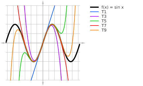
Example: Maclaurin Polynomials for sin x
Find the Maclaurin polynomials for sin x up to degree 9, and plot them on the same set of axes.
Solution
Fortunately, there is a repeating pattern in the derivatives of sin x. The derivatives repeat in blocks of four,
- sin x
- cos x
- -sin x
- -cos x
Furthermore, when you plug in x = 0, half of the Taylor coefficients will become zero because you’re plugging into sin x. The remaining terms end up alternating in sign. Keep in mind, cos 0 = 1.
| k | f(k)(x) | f(k)(1)/k! |
|---|---|---|
| 0 | f(x) = sin x | sin 0 = 0 |
| 1 | f '(x) = cos x | cos 0 = 1 |
| 2 | f ''(x) = -sin x | (-sin 0)/2! = 0 |
| 3 | f '''(x) = -cos x | (-cos 0)/3! = -1/6 |
| 4 | f(4)(x) = sin x | (sin 0)/4! = 0 |
| 5 | f(5)(x) = cos x | (cos 0)/5! = 1/120 |
| 6 | f(6)(x) = -sin x | (-sin 0)/6! = 0 |
| 7 | f(7)(x) = -cos x | (-cos 0)/7! = -1/5040 |
| 8 | f(8)(x) = sin x | (sin 0)/8! = 0 |
| 9 | f(9)(x) = cos x | (cos 0)/9! = 1/362880 |
Let’s label the Taylor polynomial of degree n by Tn. According to the table, each T2 will be the same as T1 because the degree two coefficient is zero. This is true for all of the even cases. So I’m just going to list the odd degree cases:
Below, you can see how they progressively get closer to the graph of y = sin x as the degree goes up.
What’s Next?
Taylor polynomials are just that: polynomials. And no matter how high the degree, the polynomial will not match the original function f
exactly (unless f is itself a polynomial).
Check back on this blog to see what happens when you allow the number of terms to go to infinity. Then we can get an exact match for f in a lot of cases.
These ideas are incredibly important in fields like engineering and physics. But that’s a discussion for another day!


Leave a Reply